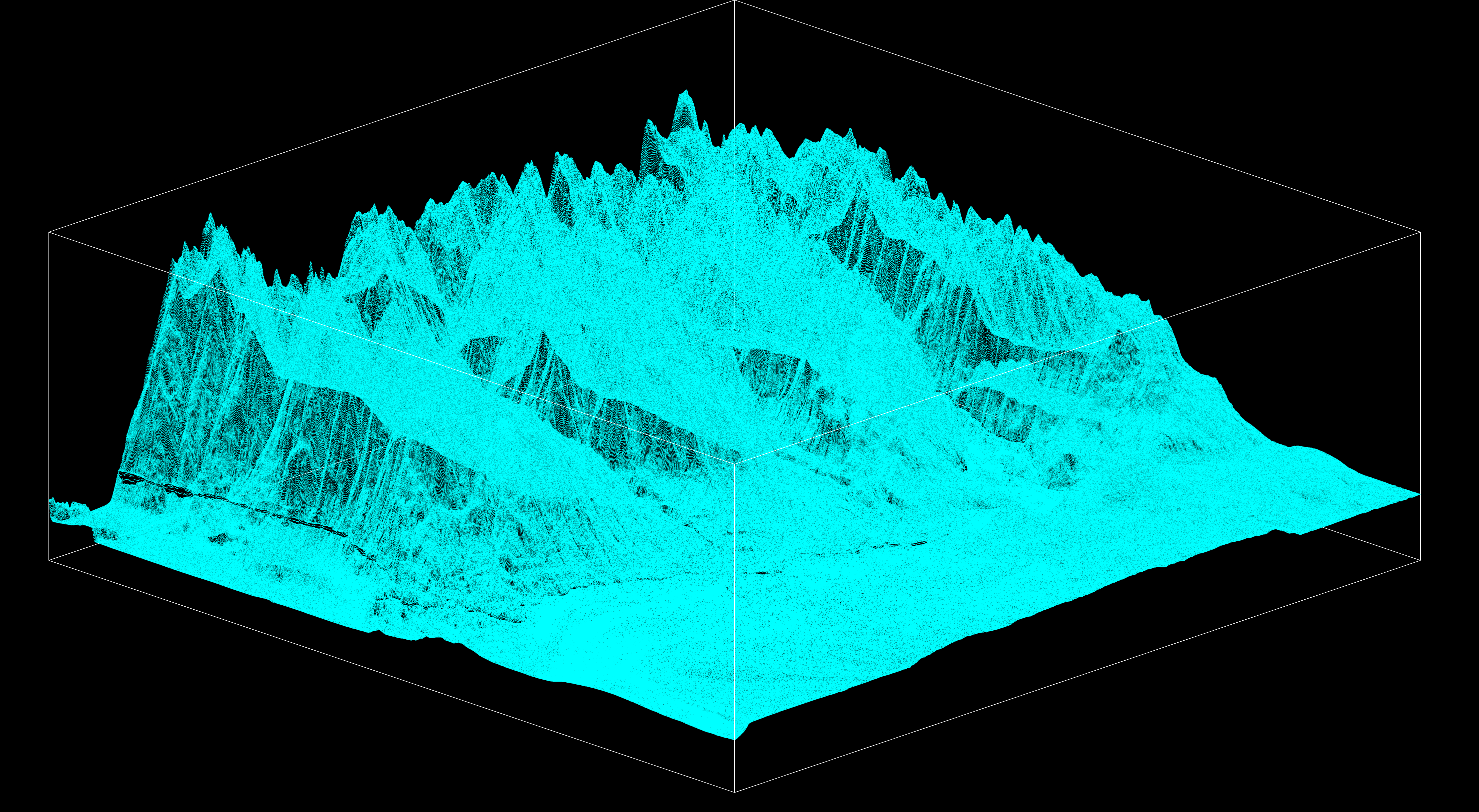
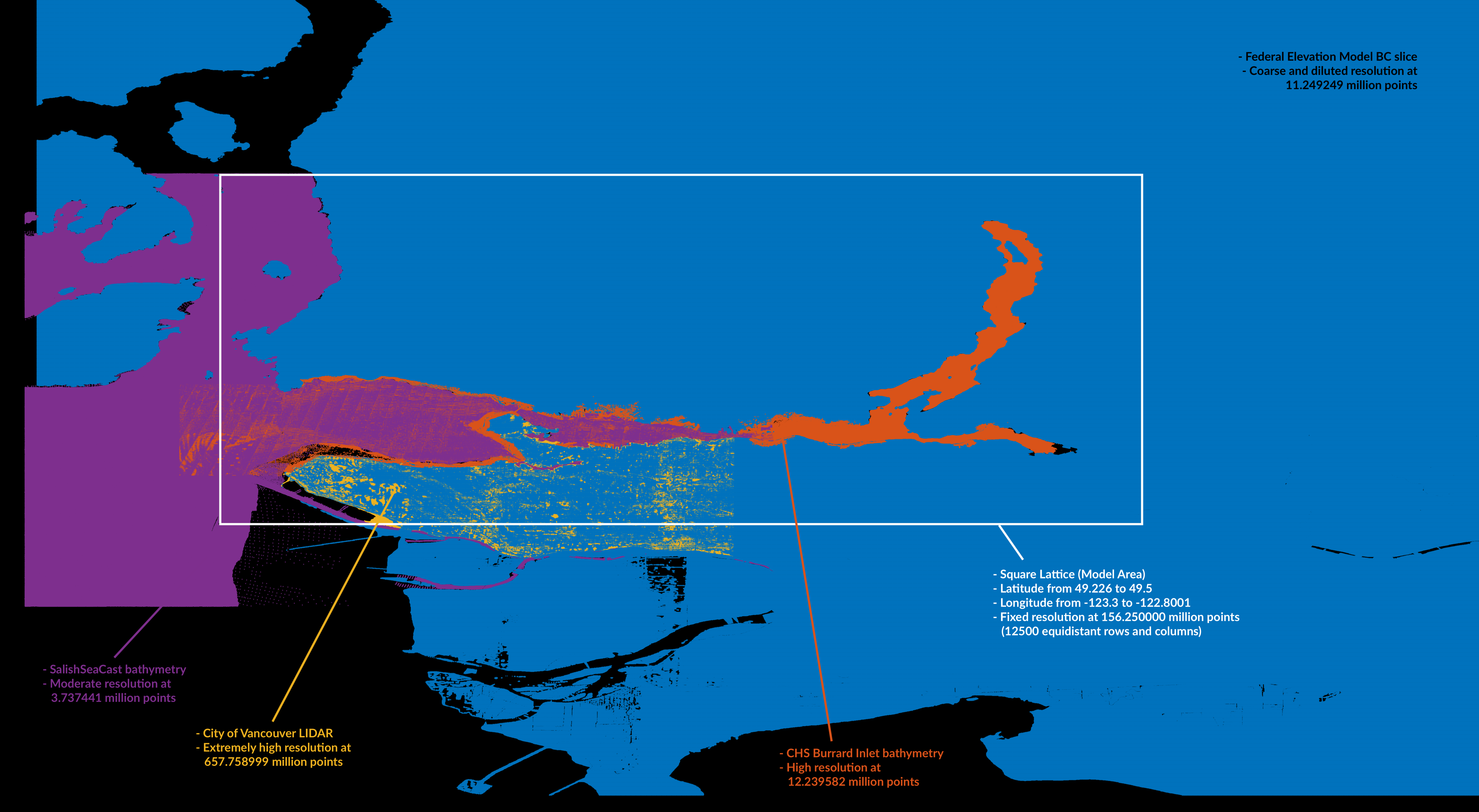
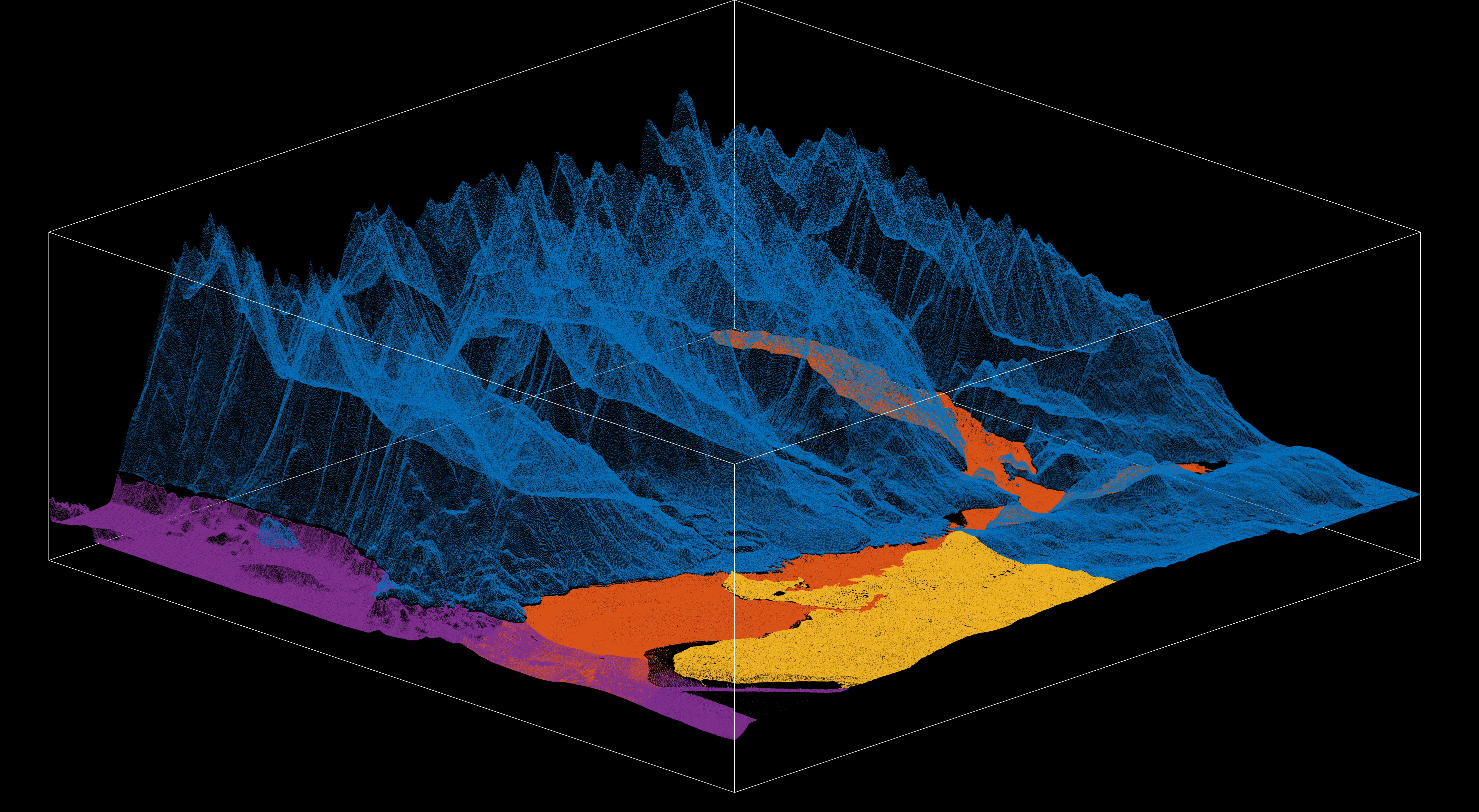
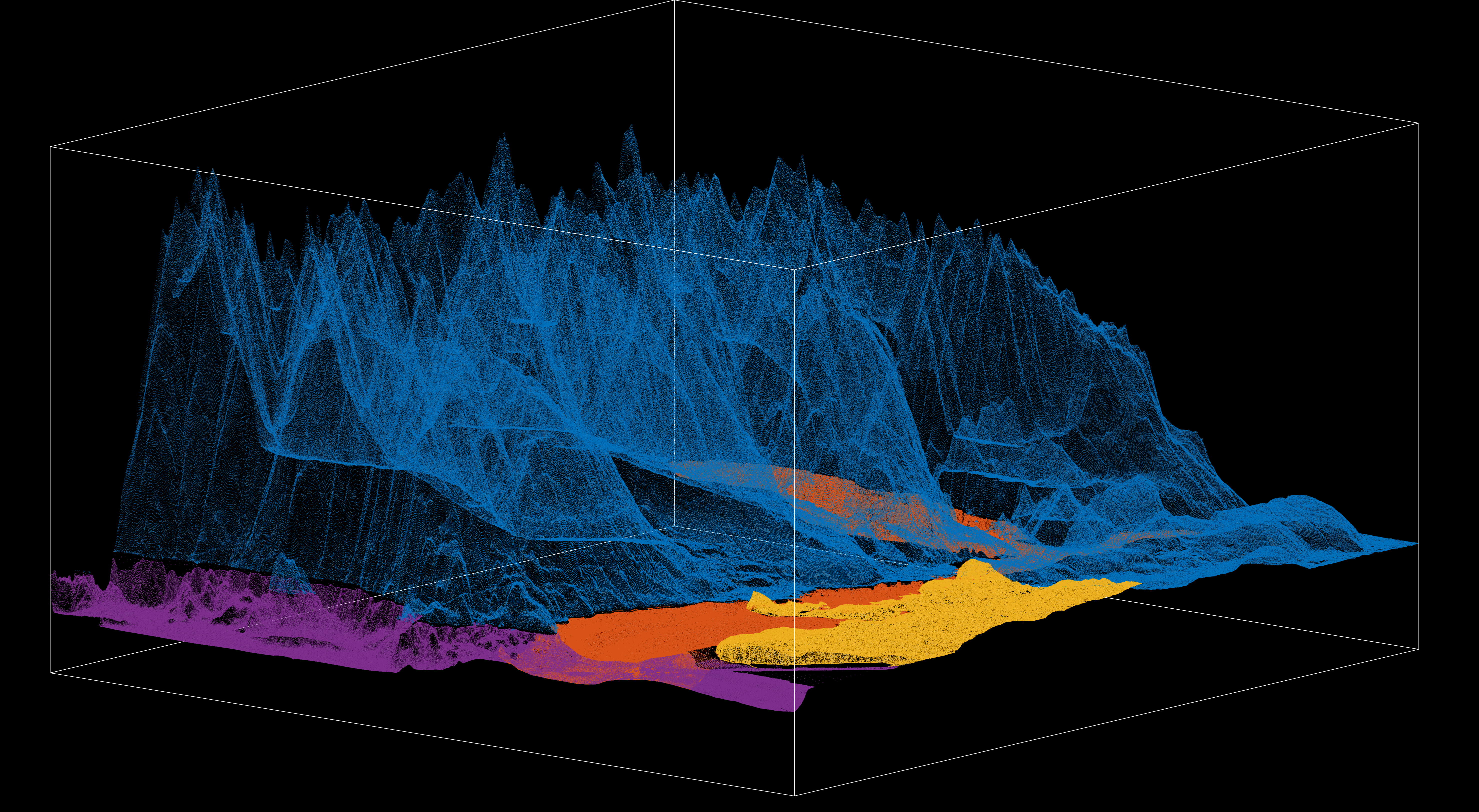
Described here is a revised pipeline that converts overlapped scattered raw point cloud datasets (sonar, bathymetry, LIDAR) into a lattice of regularly-spaced XYZ vectors. The figure below shows the raw dataset mosaic comes, which from four sources: BC slice from a Canada-wide Federal Elevation Model for dry land (Model A), CHS Burrard Inlet bathymetry (Model B), City of Vancouver LIDAR (Model C), and SalishSeaCast bathymetry (Model D). This mosaic is then sequentially mapped into a square lattice of 15000 rows and 15000 columns, a total of 225 million points.

 

 

Part 1

First we define the bounds of the lattice with latitude and longitude limits. As an initial exploration, we load the datasets to visualize their spatial extent and comparative resolutions (figure above), to get a sense of the pre-processing curation needed to minimize overlap.

% Lattice Bounds (Model Area)

Xmin=-123.3;
Xmax=-122.8;
Ymin=49.226;
Ymax=49.500;

LatticeX=[Xmin;Xmax;Xmax;Xmin;Xmin];
LatticeY=[Ymin;Ymin;Ymax;Ymax;Ymin];

% Raw source datasets

ModelA=readmatrix('AltimetryVancouver.txt');
ModelAx=ModelA(:,1);
ModelAy=ModelA(:,2);
ModelAz=ModelA(:,3);

ModelB=readmatrix('combine_5m_extract_WGS84_c.txt');
ModelBx=ModelB(:,1);
ModelBy=ModelB(:,2);
ModelBz=ModelB(:,3);

load LidarWGS_GroundX; load LidarWGS_GroundY; load LidarWGS_GroundZ
ModelCx=LidarWGS_GroundX;
ModelCy=LidarWGS_GroundY;
ModelCz=LidarWGS_GroundZ;

load SalishSeaCastExtract
ModelDx=SalishSeaCastExtract(:,1);
ModelDy=SalishSeaCastExtract(:,2);
ModelDz=SalishSeaCastExtract(:,3);

% Visualization

figure('Position',[10,10,1420,780],'Resize','off','Color','k');
hold on;axis off;axis tight;
scatter3(ModelAx,ModelAy,ModelAz,0.05);drawnow;
scatter3(ModelBx,ModelBy,ModelBz,0.05);drawnow;
scatter3(ModelCx,ModelCy,ModelCz,0.05);drawnow;
scatter3(ModelDx,ModelDy,ModelDz,0.05);drawnow;
plot3(LatticeX,LatticeY,[2000;2000;2000;2000;2000],'-w');
plot3(LatticeX,LatticeY,[-500;-500;-500;-500;-500],'-w');
plot3([Xmin;Xmin],[Ymax;Ymax],[-500,2000],'-w');
plot3([Xmax;Xmax],[Ymax;Ymax],[-500,2000],'-w');
plot3([Xmin;Xmin],[Ymin;Ymin],[-500,2000],'-w');
plot3([Xmax;Xmax],[Ymin;Ymin],[-500,2000],'-w');

 

Part 2

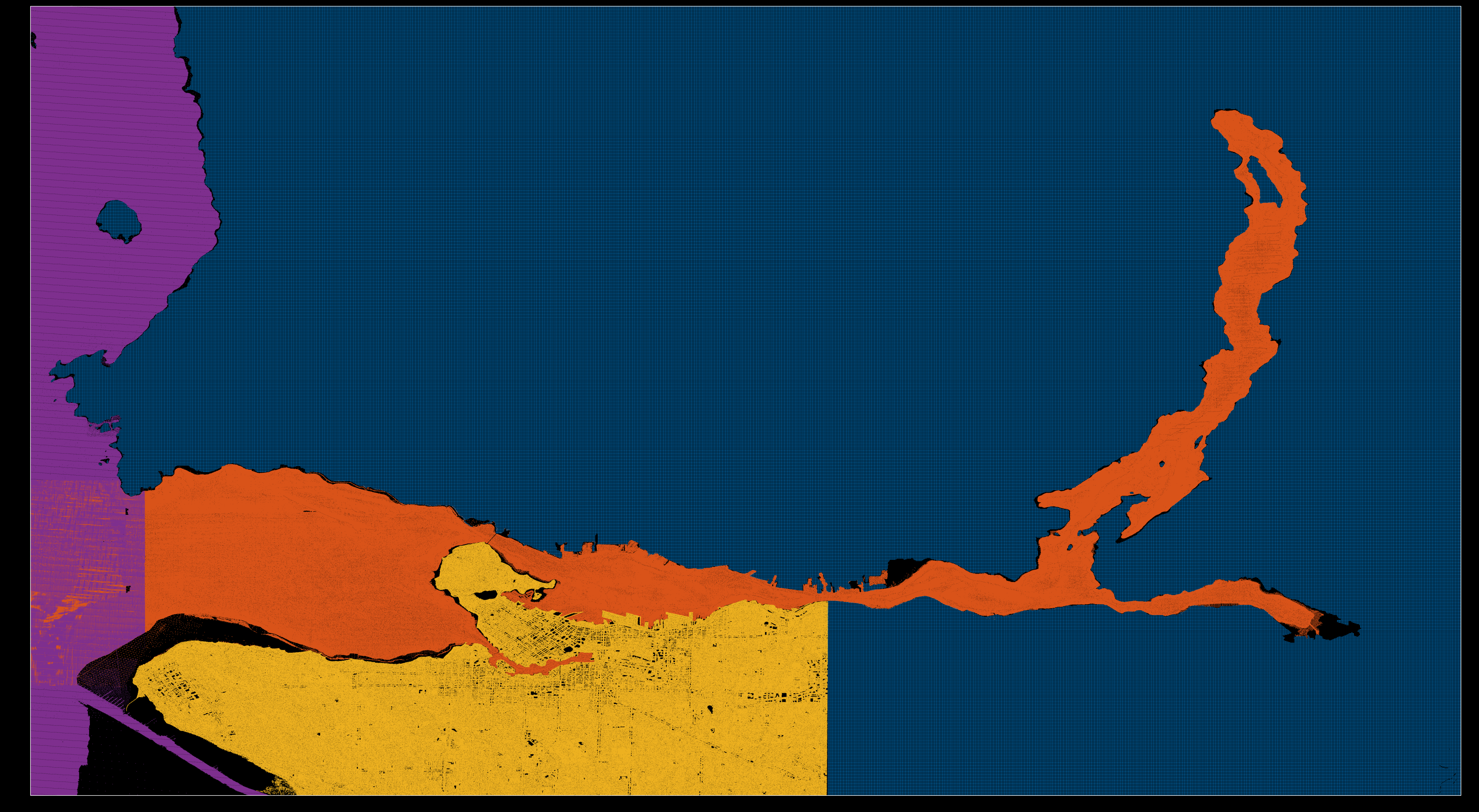
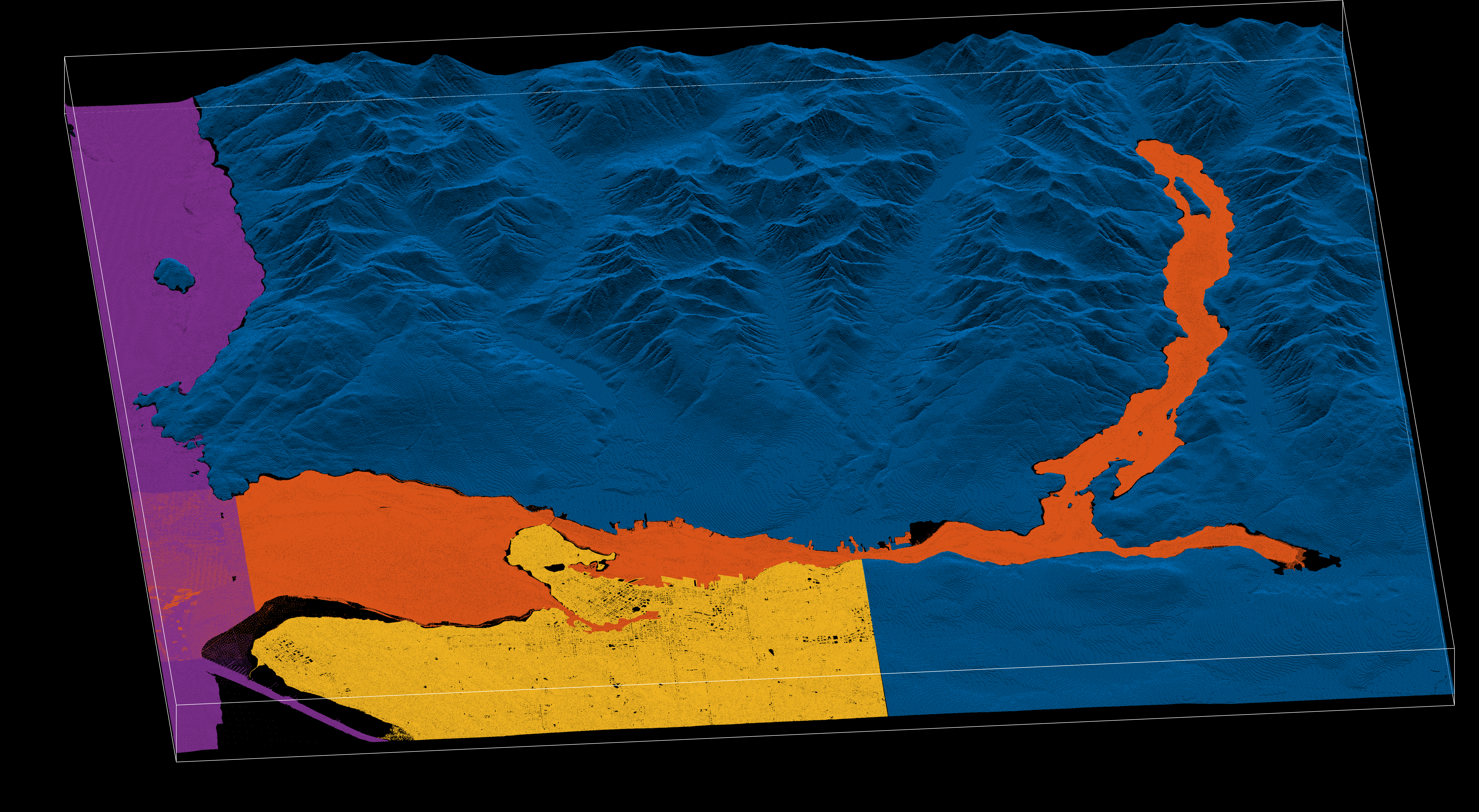
Dataset curation involves editing datasets so overlap is minimized and efficiency is maximized. The most important edit is in the Z dimension, with the 1 meter elevation contour as cutoff for elevation overlap. All datasets with above-water data will not go below 1 meter (Federal Elevation and Vancouver LIDAR altimetries), and all below-water datasets will not go above 1 meter (CHS and SalishSeaCast bathymetries). This means that the low tide contour at 0 meter will be exclusively based on bathymetric data, while the high water mark will be a hybrid (later advised by CHS ENC shapefiles). Regarding the X and Y spatial dimensions, there are specific edits to remove redundant chunks of data, with the higher-resolution dataset prevailing.

The most important edits here are for the Federal Elevation, which has the whole downtown region removed to make room for the high-resolution Vancouver LIDAR dataset. Similarly, SalishSeaCast is used for the Outer Harbour region and outskirts of the inlet, so any overlap with CHS bathymetry is removed, with CHS prevailing within the inlet region itself. Finally, because Vancouver LIDAR is an astonishingly large dataset (0.657 billion points) it is downsampled to 1/20th of its original size.

% “Model A” Federal Elevation Model BC Slice, making room for LIDAR data

ModelA=readmatrix('AltimetryVancouver.txt');
ModelAx=ModelA(:,1);
ModelAy=ModelA(:,2);
ModelAz=ModelA(:,3);
indexRemoveX=find(ModelAx<=-123.0214);
indexRemoveY=find(ModelAy<=49.2954);
indexRemove=cat(1,indexRemoveX,indexRemoveY);
[ii,~,kk]=unique(indexRemove);
freq=accumarray(kk,1);
freq(freq==1)=NaN;
indexRemove=cat(2,ii,freq);
indexRemove(any(isnan(indexRemove),2),:)=[];
ModelAx(indexRemove,1)=NaN;
ModelAy(indexRemove,1)=NaN;
indexRemoveX=find(ModelAx<=-123.1348);
indexRemoveY=find(ModelAy<=49.3147);
indexRemove=cat(1,indexRemoveX,indexRemoveY);
[ii,~,kk]=unique(indexRemove);
freq=accumarray(kk,1);
freq(freq==1)=NaN;
indexRemove=cat(2,ii,freq);
indexRemove(any(isnan(indexRemove),2),:)=[];
ModelAx(indexRemove,1)=NaN;
ModelAy(indexRemove,1)=NaN;
indexRemoveX=find(ModelAx<=-123.1125);
indexRemoveY=find(ModelAy<=49.307);
indexRemove=cat(1,indexRemoveX,indexRemoveY);
[ii,~,kk]=unique(indexRemove);
freq=accumarray(kk,1);
freq(freq==1)=NaN;
indexRemove=cat(2,ii,freq);
indexRemove(any(isnan(indexRemove),2),:)=[];
ModelAx(indexRemove,1)=NaN;
ModelAy(indexRemove,1)=NaN;
ModelAx(ModelAx<Xmin)=NaN;ModelAx(ModelAx>Xmax)=NaN;
ModelAy(ModelAy<Ymin)=NaN;ModelAy(ModelAy>Ymax)=NaN;
ModelAz(ModelAz<1)=NaN;

% “Model B” CHS Burrard Inlet bathymetry

ModelB=readmatrix('combine_5m_extract_WGS84_c.txt');
ModelBx=ModelB(:,2);ModelBx(ModelBx<Xmin)=NaN;ModelBx(ModelBx>Xmax)=NaN;
ModelBy=ModelB(:,1);ModelBy(ModelBy<Ymin)=NaN;ModelBy(ModelBy>Ymax)=NaN;
ModelBz=ModelB(:,3);ModelBz(ModelBz>1)=NaN;

% “Model C” City of Vancouver LIDAR

load LidarWGS_GroundX; load LidarWGS_GroundY; load LidarWGS_GroundZ
ModelCx=LidarWGS_GroundX;ModelCx(ModelCx<Xmin)=NaN;ModelCx(ModelCx>Xmax)=NaN;
ModelCy=LidarWGS_GroundY;ModelCy(ModelCy<Ymin)=NaN;ModelCy(ModelCy>Ymax)=NaN;
ModelCz=LidarWGS_GroundZ;ModelCz(ModelCz<1)=NaN;
NodelCx=ModelCx(1:20:end,1);
NodelCy=ModelCy(1:20:end,1);
NodelCz=ModelCz(1:20:end,1);

% “Model D” Outer Harbour from SalishSeaCast, making room for CHS batymetry

load SalishSeaCastExtract
ModelDx=SalishSeaCastExtract(:,1);
ModelDy=SalishSeaCastExtract(:,2);
ModelDz=SalishSeaCastExtract(:,3);
indexRemoveX=find(ModelDx>=-123.26);
indexRemoveY=find(ModelDy<=49.342 & ModelDy>=49.265 );
indexRemove=cat(1,indexRemoveX,indexRemoveY);
[ii,~,kk]=unique(indexRemove);
freq=accumarray(kk,1);
freq(freq==1)=NaN;
indexRemove=cat(2,ii,freq);
indexRemove(any(isnan(indexRemove),2),:)=[];
ModelDx(indexRemove,1)=NaN;
ModelDy(indexRemove,1)=NaN;
ModelDx(ModelDx<Xmin)=NaN;ModelDx(ModelDx>Xmax)=NaN;
ModelDy(ModelDy<Ymin)=NaN;ModelDy(ModelDy>Ymax)=NaN;
ModelDz(ModelDz>1)=NaN;

% Export curated XYZ datasets before lattice interpolation

X=cat(1,ModelAx,ModelBx,NodelCx,ModelDx);
Y=cat(1,ModelAy,ModelBy,NodelCy,ModelDy);
Z=cat(1,ModelAz,ModelBz,NodelCz,ModelDz);
v3MarkTwoX=X;
v3MarkTwoY=Y;
v3MarkTwoZ=Z;

 

 

Part 3

Here we remove redundancies in the XYZ vectors to further enhance efficiency before lattice interpolation. Given the large size of the curated vectors at this stage of the pipeline, this particular step can be computationally intense, so it has its own script. This step pays off by speeding up interpolation in the next step.

load v3MarkTwoX;X=v3MarkTwoX;
load v3MarkTwoY;Y=v3MarkTwoY;
load v3MarkTwoZ;Z=v3MarkTwoZ;

nansX=find(isnan(X));
nansY=find(isnan(Y));
nansZ=find(isnan(Z));

indexNaN=cat(1,nansX,nansY,nansZ);
indexNaN=unique(indexNaN);

X(indexNaN)=[];
Y(indexNaN)=[];
Z(indexNaN)=[];

MarkTwoX=X;
MarkTwoY=Y;
MarkTwoZ=Z;

 

Part 4

Finally, here we run the lattice interpolation pipeline. The K variable here is important, it determines the geometry of the kernel that assings the Z value. In detail, when K=1 the kernel assigns the instance of the nearest Z value, which can yield jitters in elevation if adjacent Z values happen to draw from the edge of another dataset that overlaps in the mosaic. This is smoothed out by K=2, which assigns the average of the two closets mosaic values, under the geometry of a 1-simplex. This can be further expanded, with K=3 using the centroid of a triangular plane or a 2-simplex, then K=4 the centroid of a tetrahedron or a 3-simplex, then K=5 the centroid of a pentachoron or a 4-simplex, and so on. Starting at K=1 or a 0-simplex, higher values of K draws a more complex kernel that smoothes out the final model. For our purposes, K=2 preserves roughness that is relevant in this region, because it’s a fjord with highly vertical rocky shores, yet K=2 still captures the mild gradients of dry land and shallower intertidal areas.

% Creating the point cloud.

load MarkTwoX; X=MarkTwoX;1
load MarkTwoY; Y=MarkTwoY;2
load MarkTwoZ; Z=MarkTwoZ;3

xyzPoints=cat(2,X,Y,zeros(length(Z),1));4
ptCloud=pointCloud(xyzPoints);5

% Creating the lattice

step=29999;
Xi=(Xmin:1/step:Xmax)';
Yi=(Ymin:0.5479999999/step:Ymax)';

string=length(Yi);
newOne=ones(string,1);
totalVector=string^2;
newX=zeros(totalVector,1);
newY=zeros(totalVector,1);

for i=1:string
    b=mod(i,100);
    if b==0
        i % Progress tracking
    end
    newX(i*string-string+1:i*string,1)=newOne.*Xi(i,1);
    newY(i*string-string+1:i*string,1)=Yi;
end

% Creating `newZ`, where the `K` variable determines smoothness

newZ=zeros(totalVector,1);

for i=1:1:totalVector
    b=mod(i,1000000);
    if b==0
        i/totalVector*100 % Progress in percent
    end
    point=[newX(i,:),newY(i,:),0];
    K=2; % A kernel in the shape of a 1-simplex
    [indices,dists]=findNearestNeighbors(ptCloud,point,K);
    pickZ=Z(indices);
    pointZ=nanmean(pickZ);
    newZ(i,1)=pointZ;
end

modelMarkTwoX=newX;
modelMarkTwoY=newY;
modelMarkTwoZ=newZ;