This code is a quick (and ugly) prototype, but it gets the job done. First we convert our input elevation array into three XYZ vectors, which in this case are loaded directly. Then we set the left-right (X), top-bottom (Y), and up-down (Z) bounds for the three-dimensional model. For Z, we know CHS set the elevation of Burrard Inlet at 0m contour to mark the lowest low tide, or sea level. However, in this case we want to capture some high tide, so the synthetic tide Z upper limit is set to 3m (this does not capture the z-jittery high water mark, but close enough). Once the Z limit is set, the remainder of the model is easy to tidy up. For X anything west of -123.2649 longitude is removed (the line between Point Atkinson and Point Grey, which amazingly is perfectly aligned north-south), and for Y anything south of 49.265 latitude is removed (anything in the model south of Point Grey). Here goes the ugly part of the code: the second round of truncation removes any Y data north of 49.35 latitude from Extract, and then combined with the main Alt dataset to complete the model. The result is a model of the drowned basin of Burrard Inlet (only).

load newX.mat
load newY.mat
load newZ.mat

tide=3;

newX(newX<-123.2649)=NaN;
newY(newY<49.265)=NaN;
newZ(newZ>tide)=NaN;

Alt=cat(2,newX,newY,newZ);
Alt(any(isnan(Alt),2),:)=[];

Extract=Alt(1:510000,:);
Alt(1:510000,:)=NaN;
Alt(any(isnan(Alt),2),:)=[];

eX=Extract(:,1);
eY=Extract(:,2);
eZ=Extract(:,3);

eY(eY>49.35)=NaN;
Extract=cat(2,eX,eY,eZ);
Extract(any(isnan(Extract),2),:)=[];

Alt=cat(1,Extract,Alt);
Alt(:,1)=rescale(Alt(:,1))*2;
Alt(:,2)=rescale(Alt(:,2));

Next, the function xyz2grid converts the XYZ vector into a non-georectified array, with the values of the elevation dimension Z distributed to each cells of the array, according to their X and Y coordinates. The function imresize is key, it converts our BurrardInlet array into a new custom aspect ratio. In this case, tweaking the aspect ratio values can yield different cell sizes, equivalent to resolution in kilometers (e.g. [2000,3000] for 10 meters, [40,60] for 500 meters).

An important note for Ecospace export, the synthetic tide Z limit is increased by 1, or tide+1, to have a buffer at-boundary data, which is later converted to NaNs and removed. Without this buffer the blocky edge of the new resolution maps will be off.

BurrardInlet=xyz2grid(Alt(:,1),Alt(:,2),Alt(:,3));
BurrardInlet=flipud(BurrardInlet);
BurrardInlet(isnan(BurrardInlet))=tide+1;

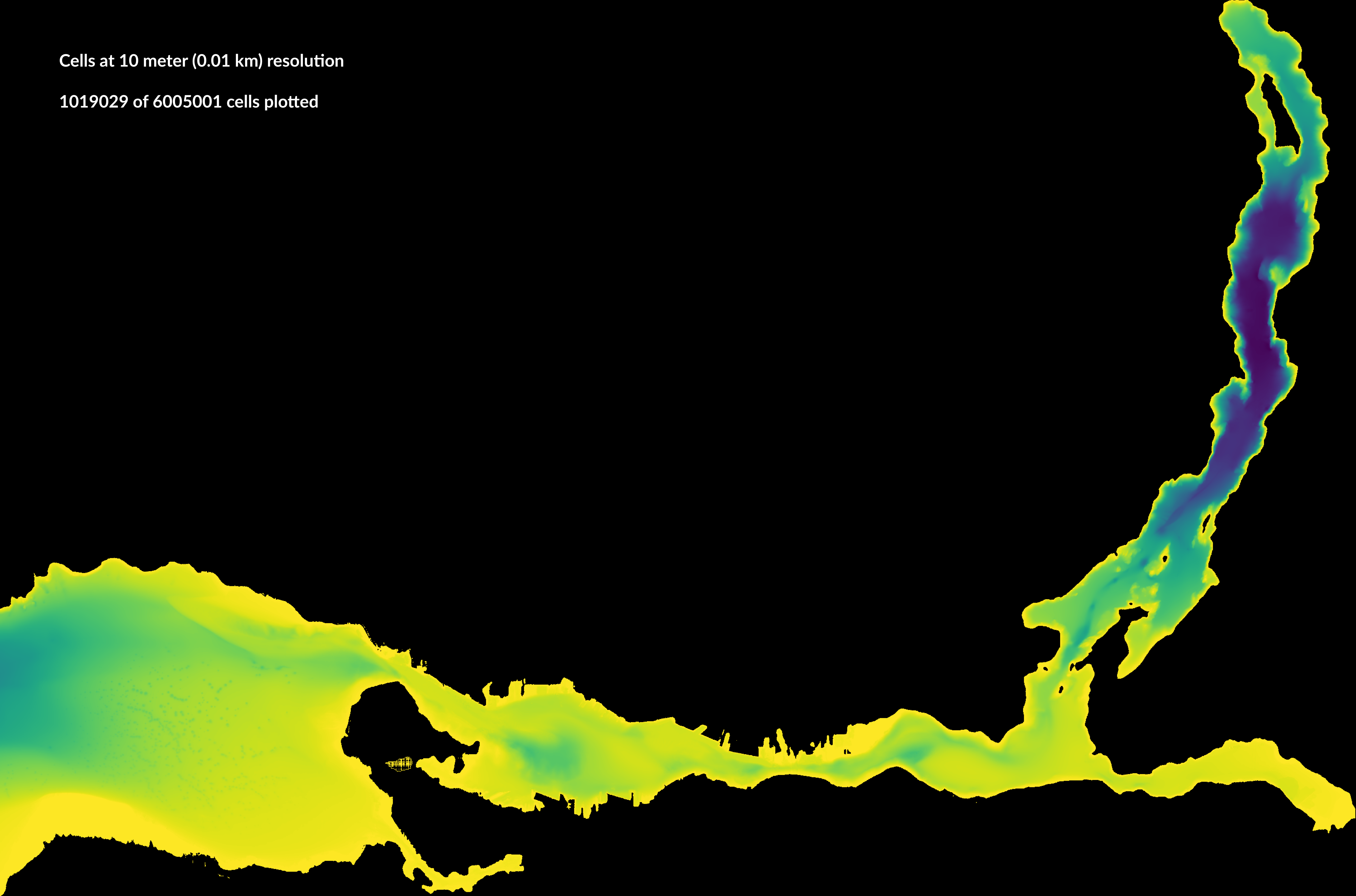
For cells at 10m (0.01 km) resolution:

A=imresize(BurrardInlet,[2000,3000]);

For cells at 100m (0.1 km) resolution:

A=imresize(BurrardInlet,[200,300]);

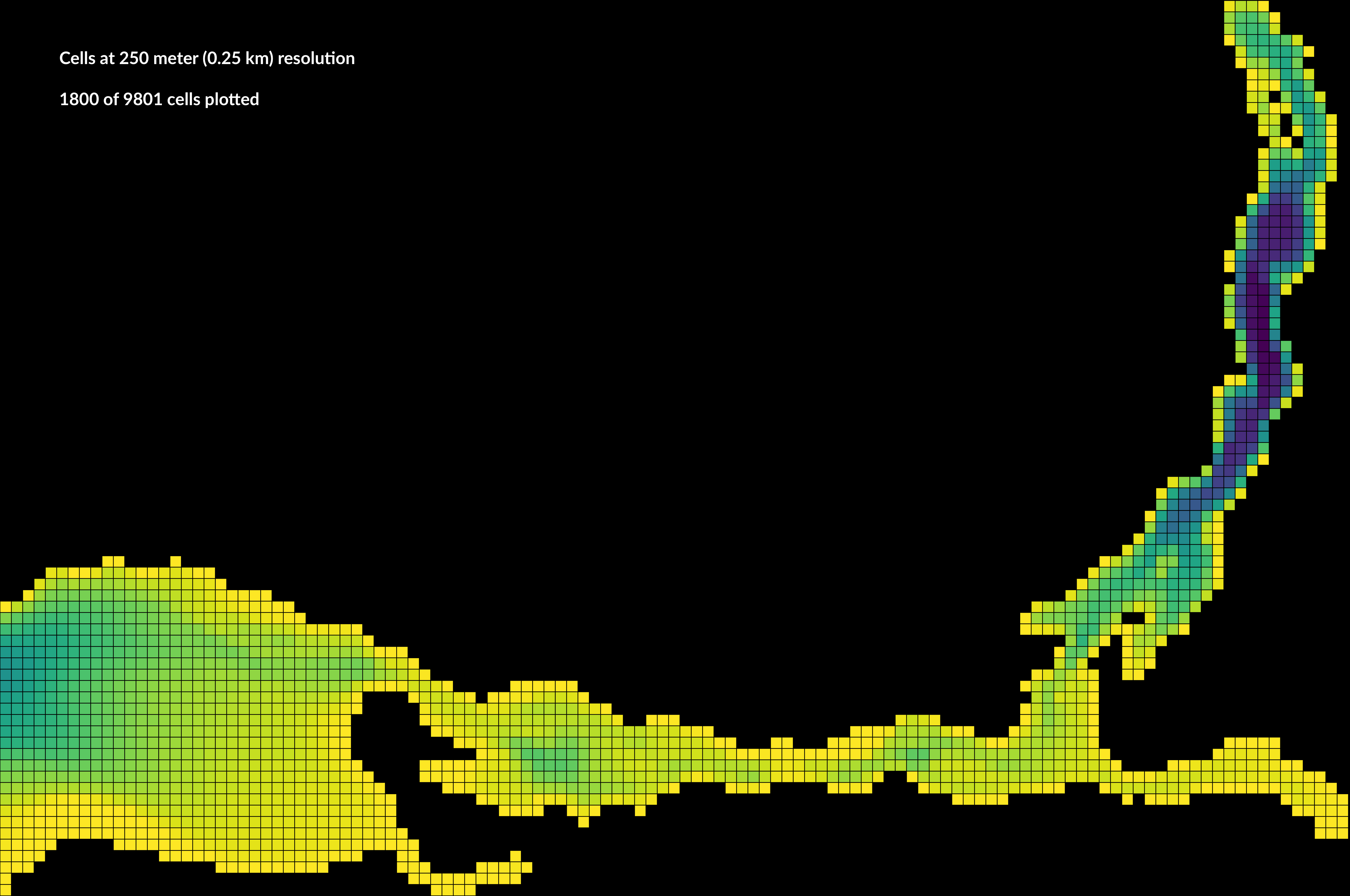
For cells at 250m (0.25 km) resolution:

A=imresize(BurrardInlet,[80,120]);

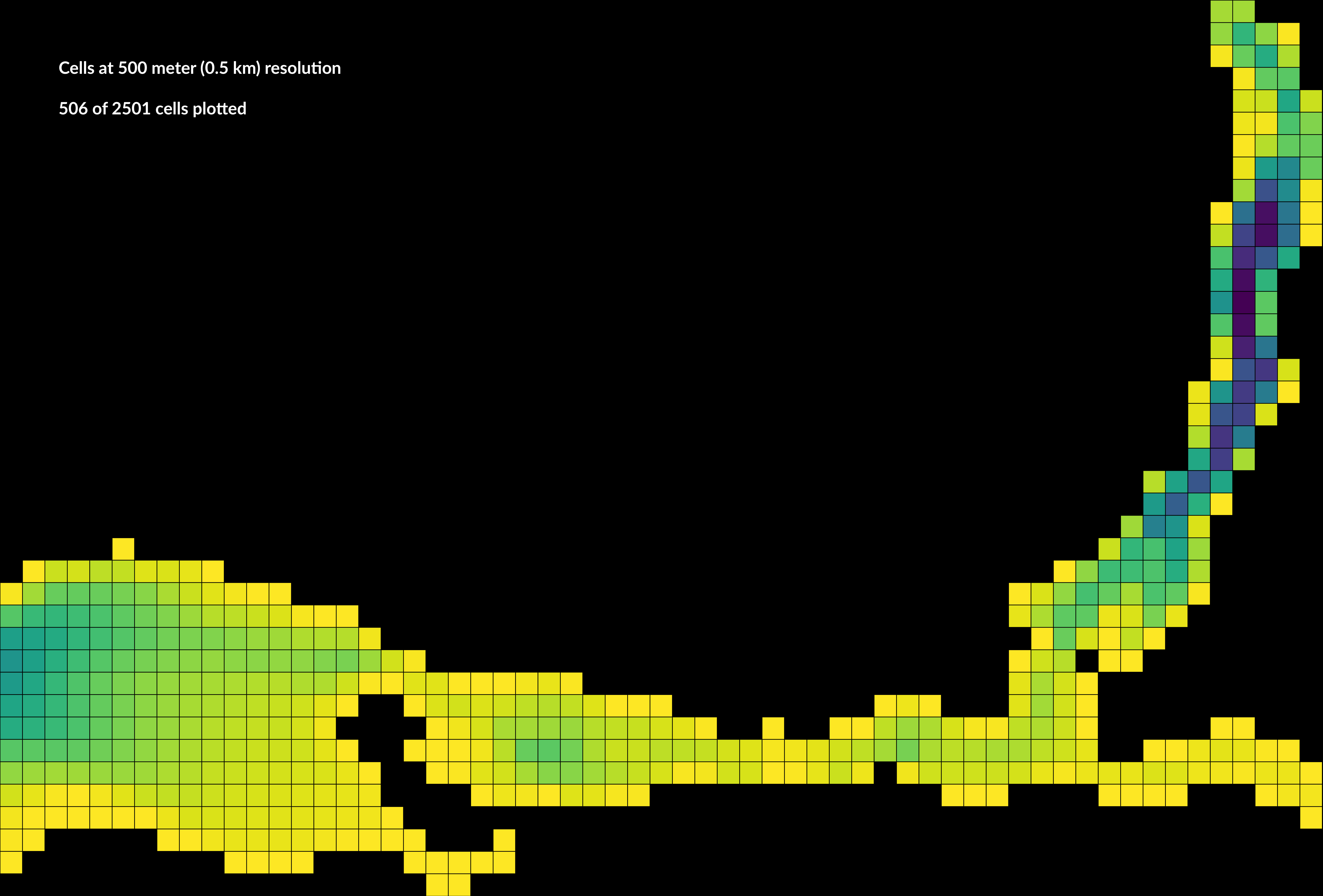
For cells at 500m (0.5 km) resolution:

A=imresize(BurrardInlet,[40,60]);

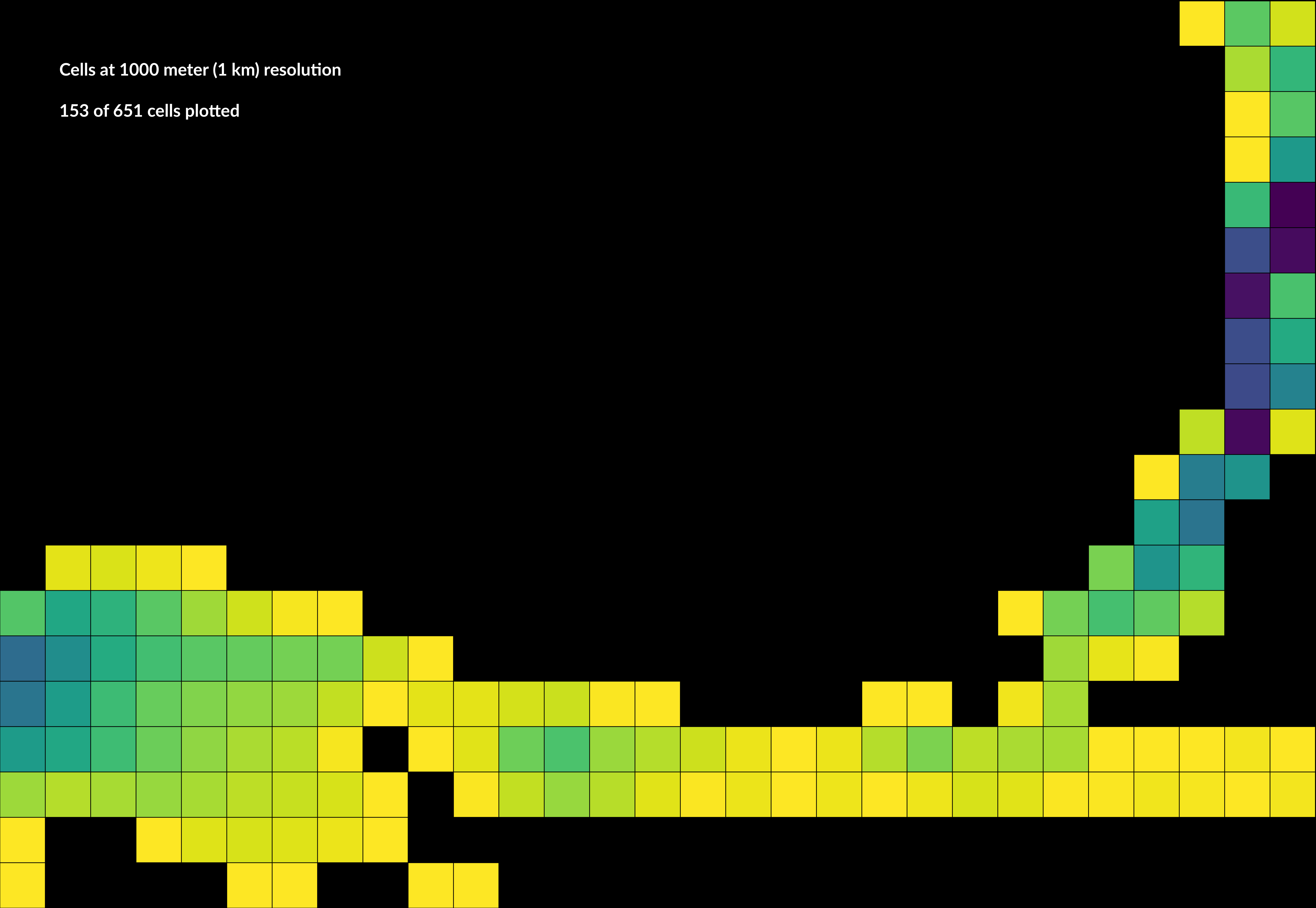
For cells at 1000m (1 km) resolution:

A=imresize(BurrardInlet,[20,30]);

To export into Ecospace-ready format, anything above tide, in this case 3 meters, is converted to NaN and then to 0 (Ecospace understands 0 elevation as land), and anything above or equal to -1 meters is converted to 1 meter (depths in Ecospace are positive, and this homogenizes the intertidal zone as the highest elevation). Important to note that Ecospace also expects “headers”, or an index vector at the first column and first row. This header must be present, else actual data will be used as a header instead, so we add synthetic headers. Finally, we convert to CSV as BurrardInlet.csv, and the last bit of code after this visualizes the arrays, figures shown below.

A(A>=tide)=NaN;A(A>=-1)=1;A=abs(A);A(isnan(A))=0;
strip=A(:,1)*0;A=cat(2,strip,A);strip=A(1,:)*0;A=cat(1,A,strip);
BurrardInlet=A;A=BurrardInlet;A(A==0)=NaN;
BurrardInlet=flipud(BurrardInlet);

writematrix(BurrardInlet,'BurrardInlet.csv');

figure('Position',[10,10,1420,780],'Resize','off','Color','k');hold on;
pcolor(BurrardInlet);shading flat;axis tight;axis equal;
axis off;colormap(flipud(viridis));