Fractals are curves with complexity and length that inversely change with measurement scale. It’s important to note that even though the natural world is full of fractals, they are not measurable physical properties of matter and energy. Fractals are geometric objects, knowing this helps explain their counterintuitive properties.

The shoreline paradox comes from attempts to measure the length of coastlines, which have fractal properties. The nooks and crannies of a shoreline can be approximated with a yardstick, which has a finite length and yields a finite total shoreline value. However, if the yardstick used decreases in length, the resolution increases, and so increases the captured fractal complexity. The solution to the paradox is not very helpful in applied science, it states that ultimately all shoreline lengths are infinite when measured without scaling compromise. The strange implication of this property is that finite surface areas in meters squared can exist in the real world, while at the same time their real perimeter in meters is infinite.

This clashes with our intuition that lengths are indeed measurable, because we know physical distances can be measured on Earth’s surface. It is through a compromise between loss of fractal information and scale resolution that shoreline length calculation is possible. Here we will explore this trade-off applied to the shoreline length of Burrard Inlet in kilometers (spoiler alert, its around 210 kilometers). Below is the shoreline of Burrard Inlet color-coded so that points closer to the start (Point Atkinson) are darker purple and points closer to the end (Point Gray) are bright yellow.

 

The code below calculates shoreline length with different yardstick lengths, defined by step. Here the step is 1000, so the total shoreline vector will be subdivided into 999 equal-length yardsticks (spoiler, mostly equal-length) that will mold into the shoreline shape. The shoreline of Burrard Inlet shown above is a 80258-by-2 vector XY, with latitude and longitude in WGS decimal format, then isolated here as variables Y and X respectively, in the code below. Given the vector has 80 thousand points, we can expect it contains lot of fractal complexity. However, knowing it has 80 thousand points does not tell the full story on resolution, because the points were not sampled to be equally spaced. The interparc function solves this, it populates the shoreline with equally spaced points, as defined by the step variable (technically pseudo-equally spaced, though this is not a problem because all distances are knowable).

 
figure('Position',[10,10,800,800],'Resize','off','Color','k');

step=1000;
XY=interparc(step,X,Y,'linear');
Q=zeros(length(XY)-1,3);

for i=1:length(XY)-1
    
    LatA=XY(i,1);LatB=XY(i+1,1);
    LonA=XY(i,2);LonB=XY(i+1,2);
    LatA=LatA/(180/pi);LatB=LatB/(180/pi);
    LonA=LonA/(180/pi);LonB=LonB/(180/pi);
    dLon=LonB-LonA;
    dLat=LatB-LatA;
    H=(sin(dLat/2)^2)+(cos(LatA)*cos(LatB)*sin(dLon/2)^2);
    H=2*asin(sqrt(H));rEarth=6371;
    Q(i,1)=dLon;
    Q(i,2)=dLat;
    Q(i,3)=H*rEarth;
    scatter(Q(:,1),Q(:,2),10,1:length(Q),'fill');

end
 
hold on;scatter(0,0,5000,'Xw');hold off;
title({['Segments: ',num2str(step)]; ...
['Total length: ',num2str(sum(Q(:,3))),' km'];' '},'Color','w');
drawnow;colormap(viridis);axis equal;axis off;
xlim([-0.04/step,+0.04/step]);ylim([-0.04/step,+0.04/step]);

The forloop that calculates distance in kilometers between any two adjacent points. The core of this forloop is the haversine formula, a trigonometric method to get the length of triangle edges on spherical surfaces, or the orthodromic distance. The forloop repeats the haversine calculation for every point pair along the shoreline, until the entire length of the XY vector is covered. The first step is to isolate points A and B and their lat and lon values, here LatA, LatB, LonA, and LonB. Then each point is converted to radians by dividing by (180/pi). It’s important to note that points A and B are immediately adjacent, with index i and index i+1. The X and Y components that explain distance between A and B are isolated in dLon and dLat. The variable H holds the result of the haversine formula, (sin(dLat/2)^2) + (cos(LatA)*cos(LatB)*sin(dLon/2)^2), followed by 2*asin(sqrt(H)). This arc length is a segment of a great circle, in this case its radius defined by a model of spherical Earth, which is 6371km. It would be wiser to use a more accurate geode model (not a perfect sphere, like WGS uses), but the region of interest is small enough, so differences in distance calculations from model to model are negligible. The variable Q is in place for plotting the results, alongside the rest of the code following the forloop. As the forloop goes, each distance in kilometers between points A and B is stored in the third column of Q, while the first two columns store th X and Y vector components, respectively, now dLon and dLat. Total shoreline length in kilometers is calculated by adding together all the values in the third column of Q. The first and second columns of Q give us, as vector definitions, each step’s direction and magnitude.

As we travel along the shoreline in equidistant steps, we expect the next point to be any cardinal direction (as the shorelinea meanders) yet with a maximum magnitude, as delimited by step. So, if all vectors plotted together, a unit circle would emerge, a distilled representation of the shoreline’s fractal complexity. The following figures show this unit circles at increasingly complex step count in powers of 10. Points closer to the start of the shoreline (Point Atkinson) are darker purple and points closer to the end of the shoreline (Point Gray) are bright yellow, and in the center is a crossmark that shows the origin, the zeroth center of the unit circle from which vector juts out.

 

 

As the step increases the yardstick dramatically decreases, and with higher resolution comes larger total length. Shown below is the asymptotic trend that results from decreasing yardstick length, which is the same as increasing the number of straight line segments, or resolution. In this case, total shoreline length for Burrard Inlet settles at around 210 kilometers.

 

 

Zooming into the section beyond the total point count of the original shoreline dataset, the length continues to increase, but at a much slower rate. Because this example is bound to the original dataset’s measurement scale, it becomes asymptotic. Rsolution cannot go higher than what the instruments used to gather the original dataset allow in the first place. In theory (and with crazy powerful instruments) we could keep measuring the shoreline with increasing complexity, so this length calculation would keep increasing, endlessly, trending towards infinity.

 

 

Here is the code for the asymptote figure above.

figure('Position',[10,10,1420,780],'Resize','off');hold on;
ylabel('Total length (kilometers)');
xlabel('Resolution (number of straight line segments)');
xline(80258,'r','Original data point count: 80258');
 
for step=100:100:1000000
    
    XY=interparc(step,X,Y,'linear');
    Q=zeros(length(XY),3);
    
    for i=1:length(XY)-1
        
        LatA=XY(i,1);LatB=XY(i+1,1);
        LonA=XY(i,2);LonB=XY(i+1,2);
        LatA=LatA/(180/pi);LatB=LatB/(180/pi);
        LonA=LonA/(180/pi);LonB=LonB/(180/pi);
        dLon=LonB-LonA;
        dLat=LatB-LatA;
        H=(sin(dLat/2)^2)+(cos(LatA)*cos(LatB)*sin(dLon/2)^2);
        H=2*asin(sqrt(H));rEarth=6371;
        Q(i,1)=dLon;
        Q(i,2)=dLat;
        Q(i,3)=H*rEarth;
        Length=sum(Q(:,3));
        
    end

    scatter(step,Length,20,'Xk');drawnow;

end

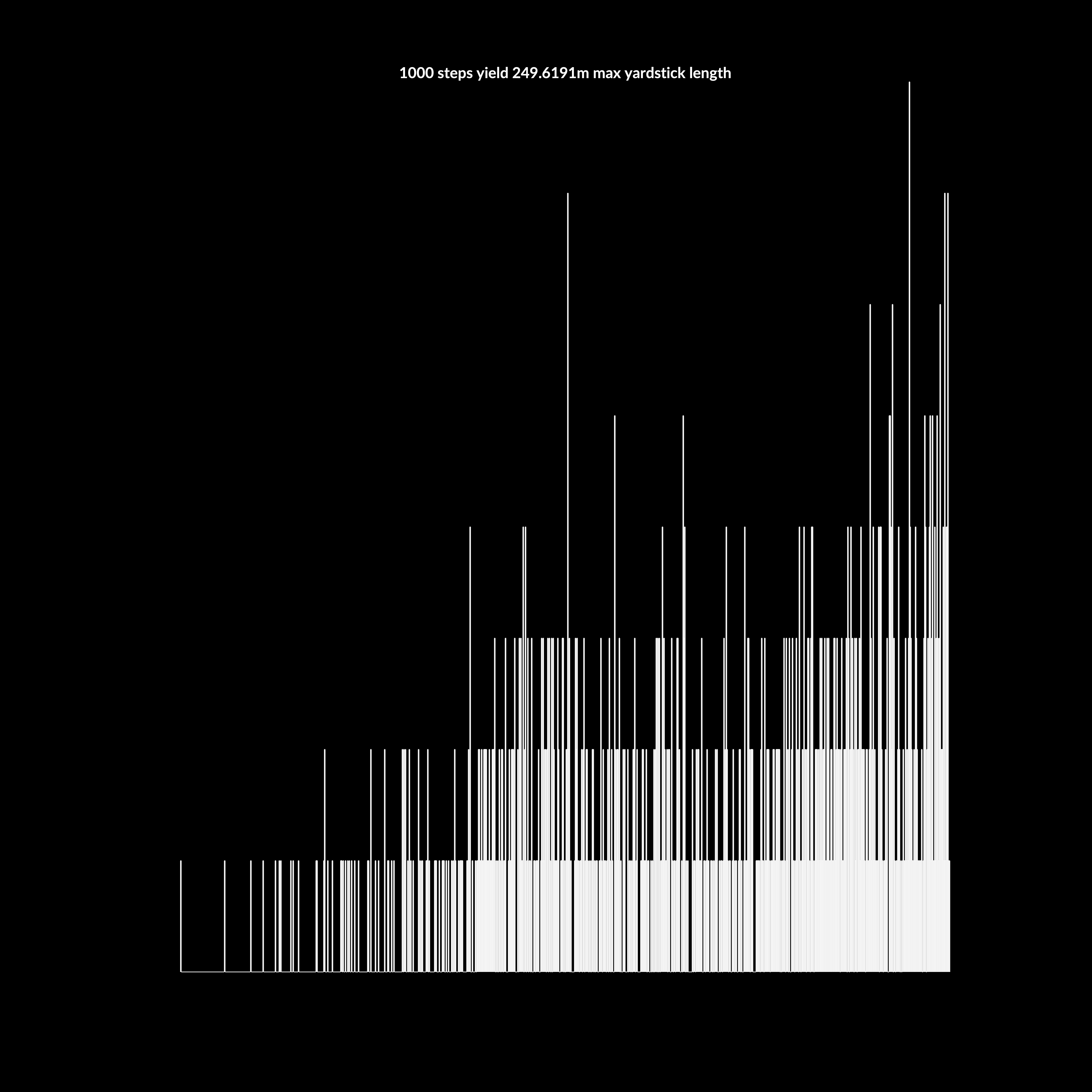
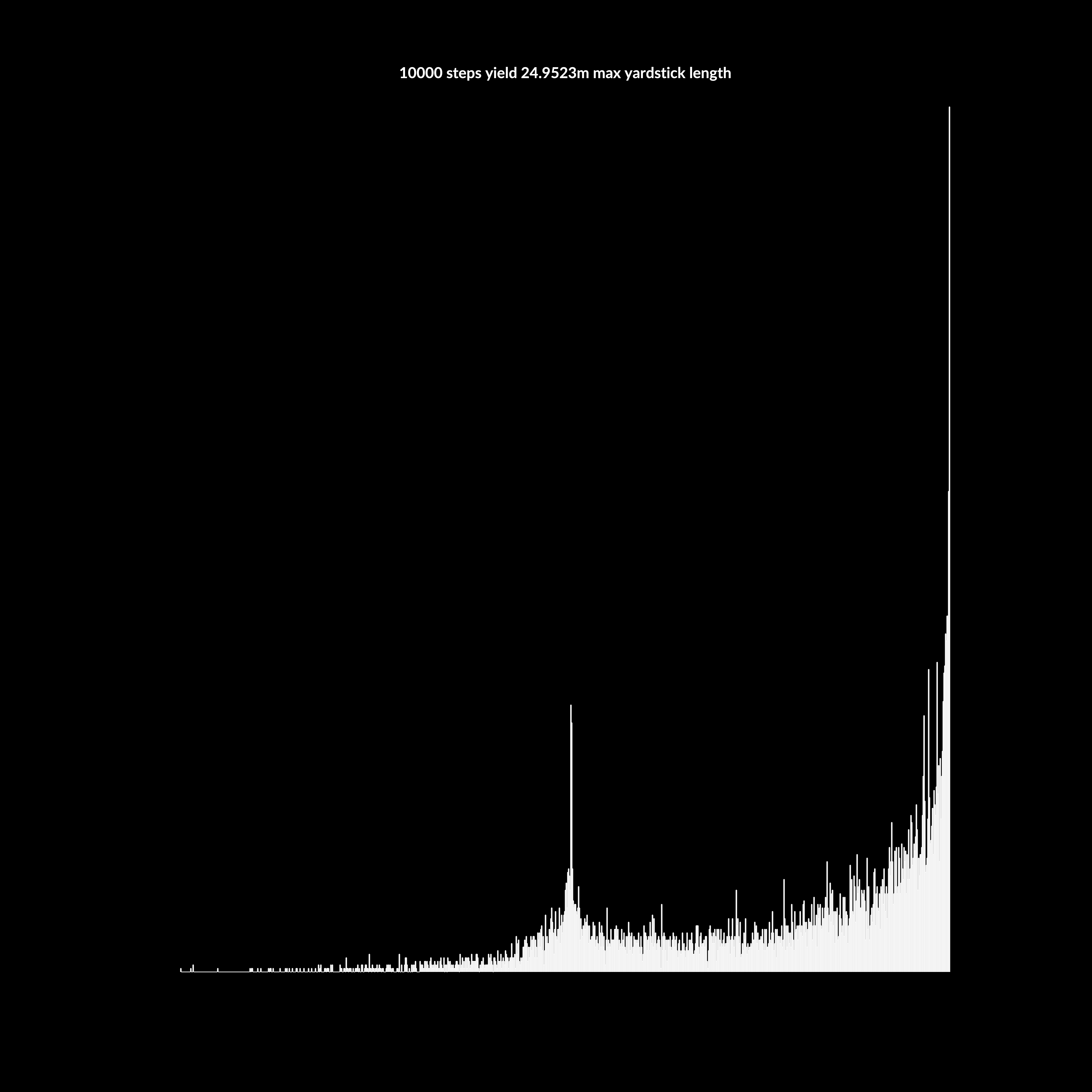
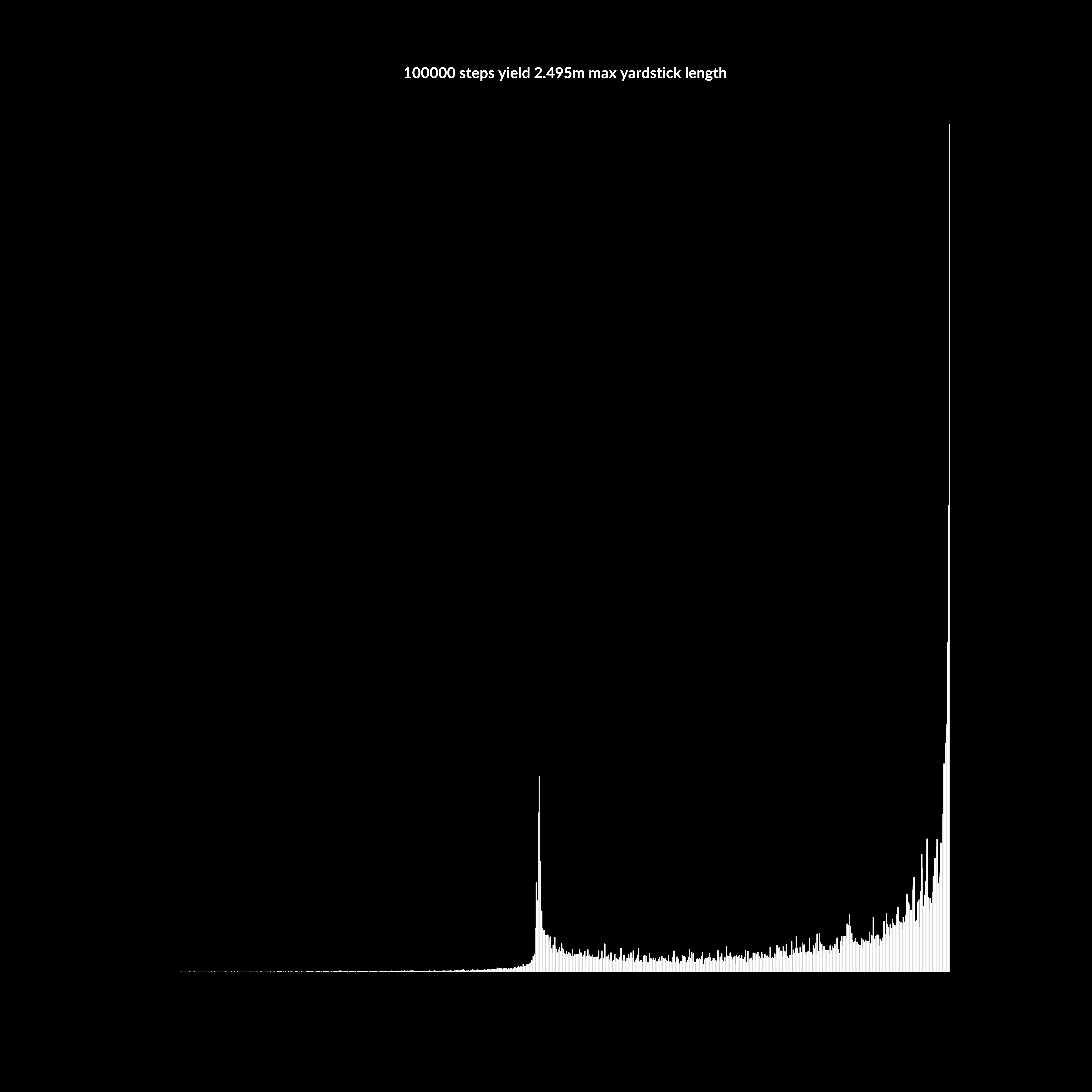
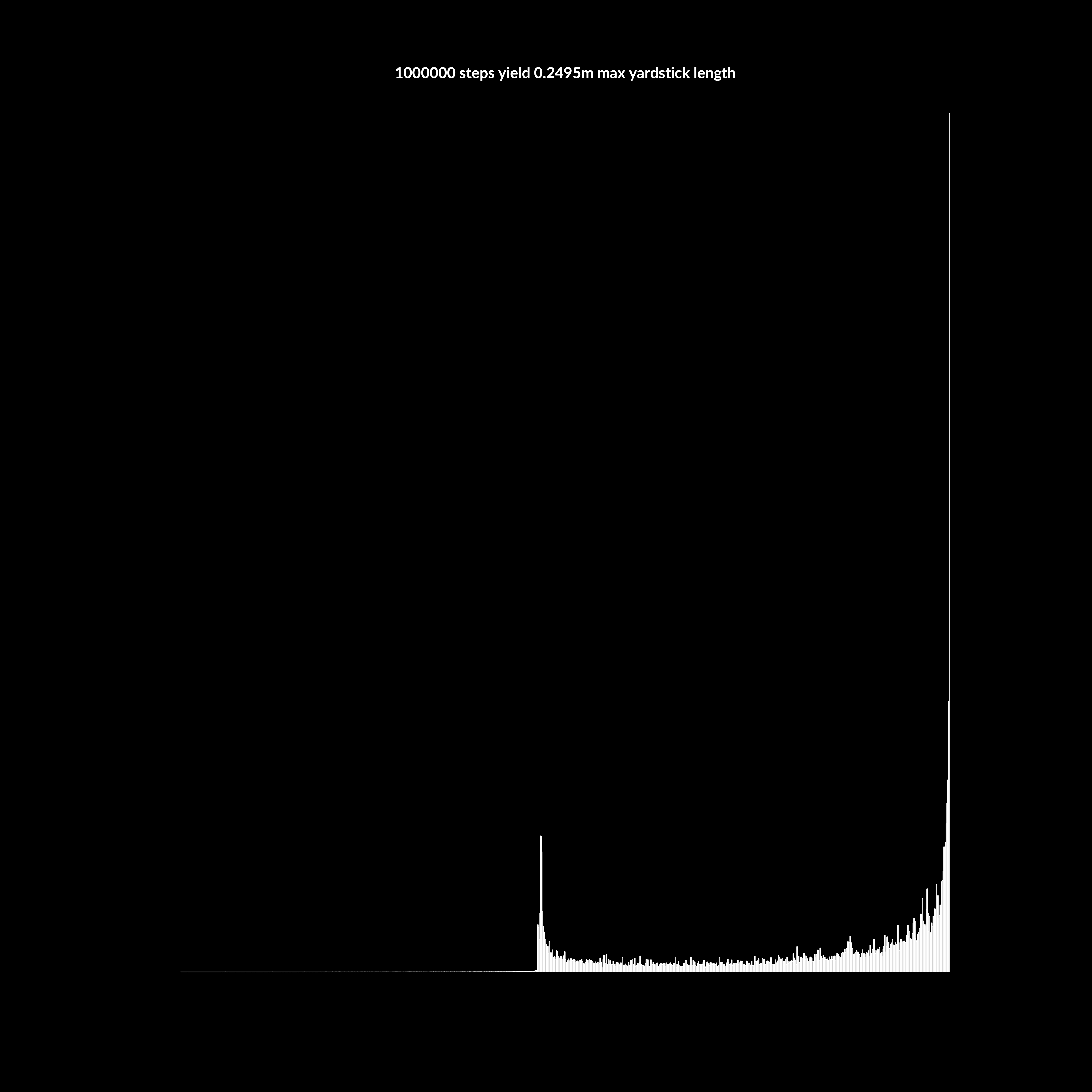
On a final note, the interparc interpolation function does yield mostly equal-length yardsticks for any given steps number, but the noise in the unit circles hints of something else going on. Below are the distribution of lengths for different steps and the length in meters of the maximum yardstick each yield. Notice that there is a cluster of yardsticks at peak length, but also at half peak length. This may be because tight curves may be too difficult to fill, so a fraction of a total yardstick is used to preserve curve complexity. This is not a problem, because all length are ultimately known. An interesting quirk of this method.