This is Matlab code that describes a method to regularize raw scattered surface data into a regular lattice. Light scans, such as sonar and LiDAR data, often are segmented into several sections, and each datapoint is irregularly scattered across the surface.

Formalizing several different datasets into a single lattice surface allows for feature visualization and analysis without the compromise of irregularly scattered data that can bias results. The six steps shown here describe a novel original method.

Step 1

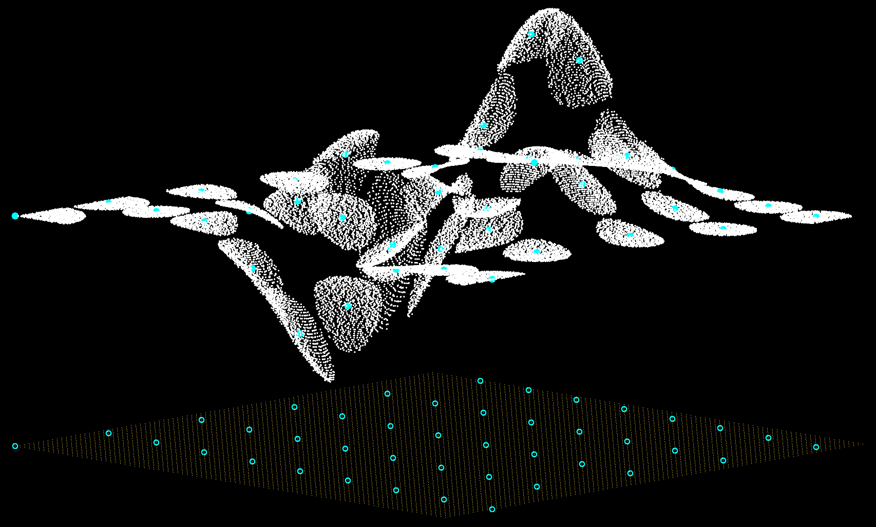
Load and compile your 3D raw data (fine if datasets spatially overlap), here called Basin, and isolate each spatial dimension into its X, Y, and Z vectors. Extract the maximum and minimum values of each vector using the nanmax and nanmin functions, these six values (two per vector) are the three-dimensional edges of the complete dataset.

X=Basin(:,1);Xmin=nanmin(X);Xmax=nanmax(X);
Y=Basin(:,2);Ymin=nanmin(Y);Ymax=nanmax(Y);
Z=Basin(:,3);Zmin=nanmin(Z);Zmax=nanmax(Z);

Step 2

The following two steps are deceitfully simple: the goal is to create a regular lattice from the known edges. First we make regularly spaced points between the edges of the X and Y dimensions, calling the new regularized vectors Xi and Yi. Then an empty vector filled with ones of length Yi is created as a placeholder for the next step.

The reciprocal of the step number is used as the determinant of length, but I haven’t figured an elegant way to connect the final vector lengths of Xi and Yi with code. The specific numbers shown here (0.5479999999:1 ratio) come from manual trial and error. It has to do with Matlab using index start at 1 instead of 0, but it works!

step=24999;
Xi=(Xmin:1/step:Xmax)';
Yi=(Ymin:0.5479999999/step:Ymax)';
string=length(Yi);
newOne=ones(string,1);

Step 3

This for-loop populates the newOne vector and turns it into a periodic newX vector for every X position in the new lattice. Simultaneously, each iteration adds a new newY value, looping across Y positions until a new X position is required. This creates an XY grid bound within the nanmax and nanmin limits of X and Y.

for i=1:string
    if i==1
        stanzaX=Xi(i,1);
        newX=newOne.*stanzaX;
        stanzaY=Yi;
        newY=stanzaY;
    else
        stanzaX=Xi(i,1);
        longX=newOne.*stanzaX;
        newX=cat(1,newX,longX);
        stanzaY=Yi;
        newY=cat(1,newY,stanzaY);
    end
end

Step 4

Creating the point cloud ptCloud, a placeholder object with all the original X and Y information and a zero dummy vector to be populated by the Z dimension, or the vector newZ.

xyzPoints=cat(2,X,Y,zeros(length(Z),1));
ptCloud=pointCloud(xyzPoints);
newZ=zeros(length(newX),1);

Step 5

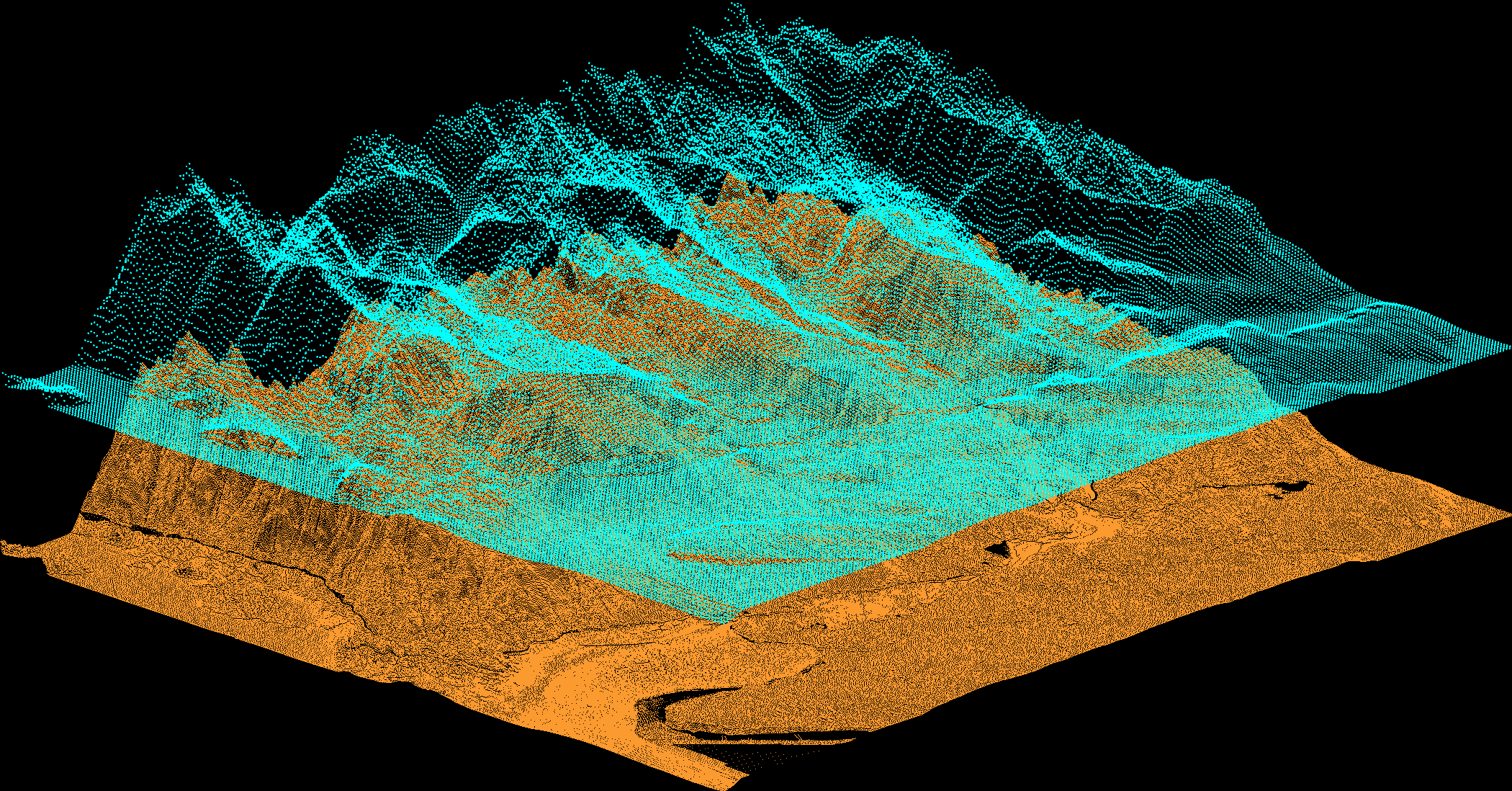
In this step everything comes together. The vector newZ gets populated by elevation data from the original X and Y data now in ptCloud using a k-nearest neighbor algorithm, here using the two closest points from the cloud and averaging them to populate the respective newZ point. This is repeated millions of times, so a modulo of every 1000000th iteration prints the i number to check progress. This step takes about 2 hours to complete, depending on how large the datasets are.

for i=1:1:length(newX)
    b=mod(i,1000000);
    	if b==0
   	i
    	end
    point=[newX(i,:),newY(i,:),0];
    K=2;
    [indices,dists]=findNearestNeighbors(ptCloud,point,K);
    pickZ=Z(indices);
    pointZ=nanmean(pickZ);
    newZ(i,1)=pointZ;
end

Step 6

Exporting into vectors, and into a final 3D vector, here called XYZ_Basin.

XYZ_Basin=cat(3,newX,newY,newZ);

 

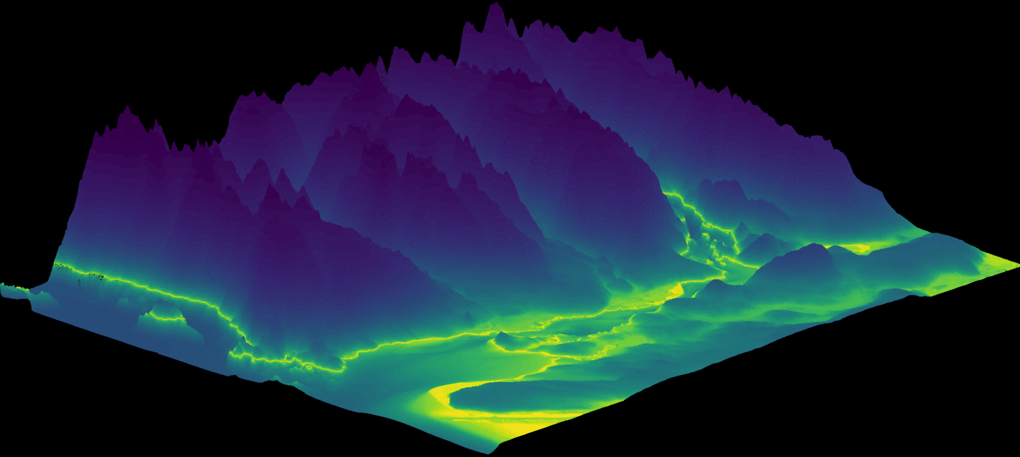
This can be exported as a .csv file (or .xyz file) for visualizations in graphical engine software. Here a hacky render is created by stithcing together several stills of the model render while slowly changing the theta angle, while the azimuth remains the same.